


Table of contents
What does L1 mean?
In Lasso Regression, we add a penalty term to the loss function during model training. The penalty term is proportional to the sum of the absolute values of the coefficients. We calculate the penalty term using the L1 norm, which is the sum of the absolute values of the individual coefficients.
Loss = MSE + λ * ||w||
here MSE is the mean squared error (for linear regression)
     λ is regularization parameter (lambda >= 0)
     ||w|| is the sum of absolutue absolute values of each coefficient.
Increasing the hyperparameter in Lasso regression aggressively shrinks coefficients towards zero, promoting higher sparsity in the model. This encourages feature selection by excluding less important features.
Implementation
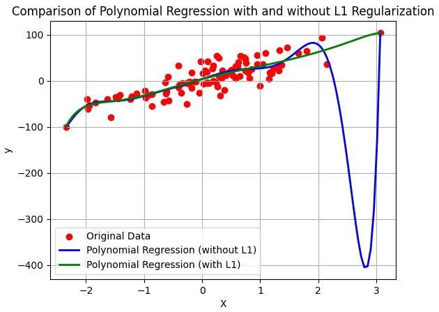
The code starts by generating a synthetic regression dataset using make_regression. Next, it applies PolynomialFeatures to create polynomial features and fits the models (linear regression without Lasso and Lasso regression) to the transformed data. Then, it plots the original data points and the fitted curves for both models. The resulting plot demonstrates the distinction in the fitted curves, emphasizing how Lasso regularization effectively controls overfitting by shrinking coefficients and promoting sparsity in the model.
import numpy as np
import matplotlib.pyplot as plt
from sklearn.preprocessing import PolynomialFeatures
from sklearn.linear_model import LinearRegression, Lasso
from sklearn.datasets import make_regression

# Generate a synthetic regression dataset with polynomial features
X, y = make_regression(n_samples=100, n_features=1, noise=20)
poly = PolynomialFeatures(degree=10)
X_poly = poly.fit_transform(X)

# Initialize and fit models
withoutL1 = LinearRegression()
withL1 = Lasso(alpha=0.1)
withoutL1.fit(X_poly, y)
withL1.fit(X_poly, y)

plt.scatter(X, y, color='red', label='Original Data')

# Predict and plot the fitted curves from withoutL1
X_plot = np.linspace(np.min(X), np.max(X), 100).reshape(-1, 1)
X_plot_poly = poly.transform(X_plot)
y_withoutL1 = withoutL1.predict(X_plot_poly)
plt.plot(X_plot, y_withoutL1, color='blue', linewidth=2, label='Polynomial Regression (without L1)')

# Predict and plot the fitted curves from withL1
y_withL1 = withL1.predict(X_plot_poly)
plt.plot(X_plot, y_withL1, color='green', linewidth=2, label='Polynomial Regression (with L1)')

# Set plot labels and legend
plt.xlabel('X')
plt.ylabel('y')
plt.legend()
plt.title('Comparison of Polynomial Regression with and without L1 Regularization')
plt.grid(True)
plt.show()
Tuning the hyperparameter
Alpha = 0.01: Potential overfitting, closely follows training data.
Alpha = 0.1: More constraints, reduces overfitting, smoother curve.
Alpha = 1.0: Balanced complexity, selects important features, captures data trend.
Alpha = 10.0: Highly constrained, potential underfitting, overly simple model.

As the hyperparameter increases, the bias of the model increases while the variance decreases.
References
Codebasics : https://www.youtube.com/watch?v=VqKq78PVO9g
Krish Naik : https://youtu.be/9lRv01HDU0s